맥OS 환경에서 RStudio에 관련된 문제 중 하나는 '한글 인코딩'입니다.

개발자가 아니라서 자세한 이유는 잘 모르지만, 


아무튼 R공부를 하는 중에 readLines()함수를 이용해 txt 파일을 불러올 때

한글이 제대로 불러와지지 않는 문제가 발생합니다.


> txt <- readLines("test.txt")

Warning message:

In readLines("test.txt") : incomplete final line found on 'test.txt'

> head(txt)

[1] "\"\xba\xb8\xb0\xed \xbdʹ\xd9"                                           

[2] "\xc0̷\xb8\xb0\xd4 \xb8\xbb\xc7ϴϱ\xee \xb4\xf5 \xba\xb8\xb0\xed \xbdʹ\xd9"

[3] "\xb3\xca\xc8\xf1 \xbb\xe7\xc1\xf8\xc0\xbb \xba\xb8\xb0\xed \xc0־"      

[4] "\xba\xb8\xb0\xed \xbdʹ\xd9"                                             

[5] "\xb3ʹ\xab \xbe\u07fc\xd3\xc7\xd1 \xbdð\xa3"                             

[6] "\xb3\xaa\xb4\xc2 \xbf츮\xb0\xa1 \xb9Ӵ\xd9" 


검색을 통해 알아낸 방법들로

파일을 불러올 때 옵션으로 인코딩을 지정한다던가,

txt 파일을 새로 만들면서 'UTF-8' 혹은 'euc-kr'으로 저장하는 방법을 사용해보기도 했지만

저는 제대로 해결되지 않았어요.


아무튼 어떻게 해결 했냐면, 일단 RStudio 자체의 인코딩 인식과 방법에 관련된 문제이지 싶어서

RStudio에서 txt 파일을 생성해 저장함으로써 간단하게 해결했습니다.


자세한 원리는 모르겠지만...

RStudio 환경에서 생성하면 사용가능한 인코딩으로 저장되지 않을까? 하는 생각으로 시도했는데 먹혀들었네요ㅎㅎ

환경설정에서 확인해 봤을 땐 system default가 UTF-8이던데

어째서 txt 파일을 UTF-8 인코딩으로 저장했을 때도 같은 문제가 발생했는지는 모르겠지만요...


Posted by Azel.Kim :

출처 : http://blog.naver.com/ilustion/220257419444


## 주성분분석

# princomp(x, cor=T) 함수를 사용

# x는 n X p 다변량 자료행렬이고, cor=T이면 상관행렬분해를, cor=F이면 공분산행렬분해를 지시

# 주성분 점수는 scores에, 주성분 부하는 loadings에 남는다

protein=read.table("J:/R을 활용한 탐색적 자료분석/protein.txt", header=TRUE)

str(protein)

'data.frame':   25 obs. of  10 variables:

 $ Country: Factor w/ 25 levels "Albania","Austria",..: 1 2 3 4 5 6 7 8 9 10 ...

 $ Beef   : num  10.1 8.9 13.5 7.8 9.7 10.6 8.4 9.5 18 10.2 ...

 $ Chicken: num  1.4 14 9.3 6 11.4 10.8 11.6 4.9 9.9 3 ...

 $ Egg    : num  0.5 4.3 4.1 1.6 2.8 3.7 3.7 2.7 3.3 2.8 ...

 $ Milk   : num  8.9 19.9 17.5 8.3 12.5 25 11.1 33.7 19.5 17.6 ...

 $ Fish   : num  0.2 2.1 4.5 1.2 2 9.9 5.4 5.8 5.7 5.9 ...

 $ Cereal : num  42.3 28 26.6 56.7 34.3 21.9 24.6 26.3 28.1 41.7 ...

 $ Potato : num  0.6 3.6 5.7 1.1 5 4.8 6.5 5.1 4.8 2.2 ...

 $ Bean   : num  5.5 1.3 2.1 3.7 1.1 0.7 0.8 1 2.4 7.8 ...

 $ Fruit  : num  1.7 4.3 4 4.2 4 2.4 3.6 1.4 6.5 6.5 ...


pca=princomp(protein[,2:10], cor=T)

names(pca)

pca$loadings[,1:2]

pca$scores[,1:2]

attach(pca)

plot(scores[,2]~scores[,1], main="Principal Component Space",

     xlim=c(-5,5), ylim=c(-5,5))

text(y=scores[,2], x=scores[,1], label=protein$Country, cex=0.8)


plot(loadings[,2]~loadings[,1], main="Principal Component Loadings",

     xlim=c(-1,1), ylim=c(-1,1))

text(y=loadings[,2], x=loadings[,1], label=colnames(protein[,2:10]),cex=0.8)

for(i in 1:9){

  arrows(0, 0, 0.8*loadings[i,1], 0.8*loadings[i,2], length=0.1)

}

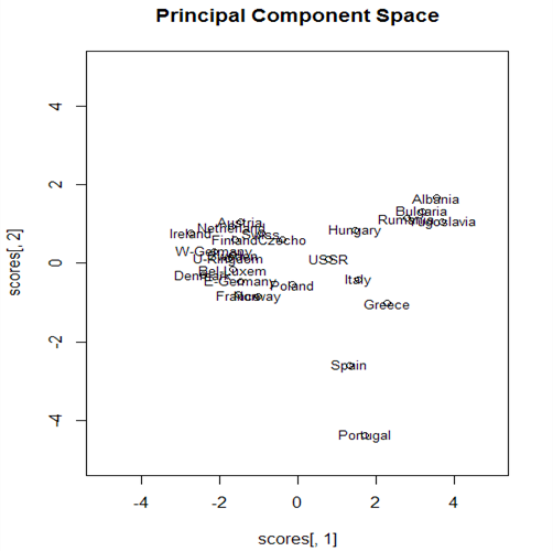
대다수의 나라들이 왼쪽에 군집을 이루가 있으나 오른쪽위에 알바니아, 불가리아, 루마니아, 유고슬라비아등 4개국이 진을 치고 있다. 관측개체 플롯내 위치와 변수 플롯의 곡류 위치가 대응하므로 이들 나라들은 곡류 섭취로 특성화된다. 아래 오른쪽에 스페인과 포르투갈이 있는데 이들은 생선, 콩, 과일 섭취로 특성화된다

그리스와 이탈리아는 콩 섭취와 관련이 깊다고 할 수 있다. 


Posted by Azel.Kim :

출처 : http://gastonsanchez.com/how-to/2012/06/17/PCA-in-R/


5 functions to do Principal Components Analysis in R

Principal Component Analysis (PCA) is a multivariate technique that allows us to summarize the systematic patterns of variations in the data.

From a data analysis standpoint, PCA is used for studying one table of observations and variables with the main idea of transforming the observed variables into a set of new variables, the principal components, which are uncorrelated and explain the variation in the data. For this reason, PCA allows to reduce a “complex” data set to a lower dimension in order to reveal the structures or the dominant types of variations in both the observations and the variables.

PCA in R

In R, there are several functions from different packages that allow us to perform PCA. In this post I’ll show you 5 different ways to do a PCA using the following functions (with their corresponding packages in parentheses):

  • prcomp() (stats)
  • princomp() (stats)
  • PCA() (FactoMineR)
  • dudi.pca() (ade4)
  • acp() (amap)

Brief note: It is no coincidence that the three external packages ("FactoMineR""ade4", and "amap") have been developed by French data analysts, which have a long tradition and preference for PCA and other related exploratory techniques.

No matter what function you decide to use, the typical PCA results should consist of a set of eigenvalues, a table with the scores or Principal Components (PCs), and a table of loadings (or correlations between variables and PCs). The eigenvalues provide information of the variability in the data. The scores provide information about the structure of the observations. The loadings (or correlations) allow you to get a sense of the relationships between variables, as well as their associations with the extracted PCs.

The Data

To make things easier, we’ll use the dataset USArrests that already comes with R. It’s a data frame with 50 rows (USA states) and 4 columns containing information about violent crime rates by US State. Since most of the times the variables are measured in different scales, the PCA must be performed with standardized data (mean = 0, variance = 1). The good news is that all of the functions that perform PCA come with parameters to specify that the analysis must be applied on standardized data.

Option 1: using prcomp()

The function prcomp() comes with the default "stats"package, which means that you don’t have to install anything. It is perhaps the quickest way to do a PCA if you don’t want to install other packages.

# PCA with function prcomp
pca1 = prcomp(USArrests, scale. = TRUE)

# sqrt of eigenvalues
pca1$sdev
## [1] 1.5749 0.9949 0.5971 0.4164
# loadings
head(pca1$rotation)
##              PC1     PC2     PC3      PC4
## Murder   -0.5359  0.4182 -0.3412  0.64923
## Assault  -0.5832  0.1880 -0.2681 -0.74341
## UrbanPop -0.2782 -0.8728 -0.3780  0.13388
## Rape     -0.5434 -0.1673  0.8178  0.08902
# PCs (aka scores)
head(pca1$x)
##                PC1     PC2      PC3      PC4
## Alabama    -0.9757  1.1220 -0.43980  0.15470
## Alaska     -1.9305  1.0624  2.01950 -0.43418
## Arizona    -1.7454 -0.7385  0.05423 -0.82626
## Arkansas    0.1400  1.1085  0.11342 -0.18097
## California -2.4986 -1.5274  0.59254 -0.33856
## Colorado   -1.4993 -0.9776  1.08400  0.00145

Option 2: using princomp()

The function princomp() also comes with the default "stats" package, and it is very similar to her cousin prcomp(). What I don’t like of princomp() is that sometimes it won’t display all the values for the loadings, but this is a minor detail.

# PCA with function princomp
pca2 = princomp(USArrests, cor = TRUE)

# sqrt of eigenvalues
pca2$sdev
## Comp.1 Comp.2 Comp.3 Comp.4 
## 1.5749 0.9949 0.5971 0.4164
# loadings
unclass(pca2$loadings)
##           Comp.1  Comp.2  Comp.3   Comp.4
## Murder   -0.5359  0.4182 -0.3412  0.64923
## Assault  -0.5832  0.1880 -0.2681 -0.74341
## UrbanPop -0.2782 -0.8728 -0.3780  0.13388
## Rape     -0.5434 -0.1673  0.8178  0.08902
# PCs (aka scores)
head(pca2$scores)
##             Comp.1  Comp.2   Comp.3    Comp.4
## Alabama    -0.9856  1.1334 -0.44427  0.156267
## Alaska     -1.9501  1.0732  2.04000 -0.438583
## Arizona    -1.7632 -0.7460  0.05478 -0.834653
## Arkansas    0.1414  1.1198  0.11457 -0.182811
## California -2.5240 -1.5429  0.59856 -0.341996
## Colorado   -1.5146 -0.9876  1.09501  0.001465

Option 3: using PCA()

A highly recommended option, especially if you want more detailed results and assessing tools, is the PCA() function from the package "FactoMineR". It is by far the best PCA function in R and it comes with a number of parameters that allow you to tweak the analysis in a very nice way.

# PCA with function PCA
library(FactoMineR)

# apply PCA
pca3 = PCA(USArrests, graph = FALSE)

# matrix with eigenvalues
pca3$eig
##        eigenvalue percentage of variance cumulative percentage of variance
## comp 1     2.4802                 62.006                             62.01
## comp 2     0.9898                 24.744                             86.75
## comp 3     0.3566                  8.914                             95.66
## comp 4     0.1734                  4.336                            100.00
# correlations between variables and PCs
pca3$var$coord
##           Dim.1   Dim.2   Dim.3    Dim.4
## Murder   0.8440 -0.4160  0.2038  0.27037
## Assault  0.9184 -0.1870  0.1601 -0.30959
## UrbanPop 0.4381  0.8683  0.2257  0.05575
## Rape     0.8558  0.1665 -0.4883  0.03707
# PCs (aka scores)
head(pca3$ind$coord)
##              Dim.1   Dim.2    Dim.3     Dim.4
## Alabama     0.9856 -1.1334  0.44427  0.156267
## Alaska      1.9501 -1.0732 -2.04000 -0.438583
## Arizona     1.7632  0.7460 -0.05478 -0.834653
## Arkansas   -0.1414 -1.1198 -0.11457 -0.182811
## California  2.5240  1.5429 -0.59856 -0.341996
## Colorado    1.5146  0.9876 -1.09501  0.001465

Option 4: using dudi.pca()

Another option is to use the dudi.pca() function from the package "ade4" which has a huge amount of other methods as well as some interesting graphics.

# PCA with function dudi.pca
library(ade4)

# apply PCA
pca4 = dudi.pca(USArrests, nf = 5, scannf = FALSE)

# eigenvalues
pca4$eig
## [1] 2.4802 0.9898 0.3566 0.1734
# loadings
pca4$c1
##              CS1     CS2     CS3      CS4
## Murder   -0.5359  0.4182 -0.3412  0.64923
## Assault  -0.5832  0.1880 -0.2681 -0.74341
## UrbanPop -0.2782 -0.8728 -0.3780  0.13388
## Rape     -0.5434 -0.1673  0.8178  0.08902
# correlations between variables and PCs
pca4$co
##            Comp1   Comp2   Comp3    Comp4
## Murder   -0.8440  0.4160 -0.2038  0.27037
## Assault  -0.9184  0.1870 -0.1601 -0.30959
## UrbanPop -0.4381 -0.8683 -0.2257  0.05575
## Rape     -0.8558 -0.1665  0.4883  0.03707
# PCs
head(pca4$li)
##              Axis1   Axis2    Axis3     Axis4
## Alabama    -0.9856  1.1334 -0.44427  0.156267
## Alaska     -1.9501  1.0732  2.04000 -0.438583
## Arizona    -1.7632 -0.7460  0.05478 -0.834653
## Arkansas    0.1414  1.1198  0.11457 -0.182811
## California -2.5240 -1.5429  0.59856 -0.341996
## Colorado   -1.5146 -0.9876  1.09501  0.001465

Option 5: using acp()

A fifth possibility is the acp() function from the package "amap".

# PCA with function acp
library(amap)

# apply PCA
pca5 = acp(USArrests)

# sqrt of eigenvalues
pca5$sdev
## Comp 1 Comp 2 Comp 3 Comp 4 
## 1.5749 0.9949 0.5971 0.4164
# loadings
pca5$loadings
##          Comp 1  Comp 2  Comp 3   Comp 4
## Murder   0.5359  0.4182 -0.3412  0.64923
## Assault  0.5832  0.1880 -0.2681 -0.74341
## UrbanPop 0.2782 -0.8728 -0.3780  0.13388
## Rape     0.5434 -0.1673  0.8178  0.08902
# scores
head(pca5$scores)
##             Comp 1  Comp 2   Comp 3   Comp 4
## Alabama     0.9757  1.1220 -0.43980  0.15470
## Alaska      1.9305  1.0624  2.01950 -0.43418
## Arizona     1.7454 -0.7385  0.05423 -0.82626
## Arkansas   -0.1400  1.1085  0.11342 -0.18097
## California  2.4986 -1.5274  0.59254 -0.33856
## Colorado    1.4993 -0.9776  1.08400  0.00145

Of course these are not the only options to do a PCA, but I’ll leave the other approaches for another post.

PCA plots

Everybody uses PCA to visualize the data, and most of the discussed functions come with their own plot functions. But you can also make use of the great graphical displays of "ggplot2". Just to show you a couple of plots, let’s take the basic results from prcomp().

Plot of observations

# load ggplot2
library(ggplot2)

# create data frame with scores
scores = as.data.frame(pca1$x)

# plot of observations
ggplot(data = scores, aes(x = PC1, y = PC2, label = rownames(scores))) +
  geom_hline(yintercept = 0, colour = "gray65") +
  geom_vline(xintercept = 0, colour = "gray65") +
  geom_text(colour = "tomato", alpha = 0.8, size = 4) +
  ggtitle("PCA plot of USA States - Crime Rates")

center

Circle of correlations

# function to create a circle
circle <- function(center = c(0, 0), npoints = 100) {
    r = 1
    tt = seq(0, 2 * pi, length = npoints)
    xx = center[1] + r * cos(tt)
    yy = center[1] + r * sin(tt)
    return(data.frame(x = xx, y = yy))
}
corcir = circle(c(0, 0), npoints = 100)

# create data frame with correlations between variables and PCs
correlations = as.data.frame(cor(USArrests, pca1$x))

# data frame with arrows coordinates
arrows = data.frame(x1 = c(0, 0, 0, 0), y1 = c(0, 0, 0, 0), x2 = correlations$PC1, 
    y2 = correlations$PC2)

# geom_path will do open circles
ggplot() + geom_path(data = corcir, aes(x = x, y = y), colour = "gray65") + 
    geom_segment(data = arrows, aes(x = x1, y = y1, xend = x2, yend = y2), colour = "gray65") + 
    geom_text(data = correlations, aes(x = PC1, y = PC2, label = rownames(correlations))) + 
    geom_hline(yintercept = 0, colour = "gray65") + geom_vline(xintercept = 0, 
    colour = "gray65") + xlim(-1.1, 1.1) + ylim(-1.1, 1.1) + labs(x = "pc1 aixs", 
    y = "pc2 axis") + ggtitle("Circle of correlations")

center


Posted by Azel.Kim :

출처 : https://stat.ethz.ch/pipermail/r-help/2007-February/125860.html


[R] Randomly extract rows from a data frame

Using the 'iris' dataset in R: # Select 2 random rows > iris[sample(nrow(iris), 2), ] Sepal.Length Sepal.Width Petal.Length Petal.Width Species 96 5.7 3.0 4.2 1.2 versicolor 17 5.4 3.9 1.3 0.4 setosa # Select 5 random rows > iris[sample(nrow(iris), 5), ] Sepal.Length Sepal.Width Petal.Length Petal.Width Species 83 5.8 2.7 3.9 1.2 versicolor 12 4.8 3.4 1.6 0.2 setosa 63 6.0 2.2 4.0 1.0 versicolor 80 5.7 2.6 3.5 1.0 versicolor 49 5.3 3.7 1.5 0.2 setosa


Posted by Azel.Kim :

R studio 단축키

2016. 10. 9. 16:24 from 통계/R

출처 : https://support.rstudio.com/hc/en-us/articles/200711853-Keyboard-Shortcuts


Keyboard Shortcuts


This information is available directly in the RStudio IDE under the Tools menu:

Tools → Keyboard Shortcuts Help.


Console

DescriptionWindows & LinuxMac
Move cursor to ConsoleCtrl+2Ctrl+2
Clear consoleCtrl+LCtrl+L
Move cursor to beginning of lineHomeCommand+Left
Move cursor to end of lineEndCommand+Right
Navigate command historyUp/DownUp/Down
Popup command historyCtrl+UpCommand+Up
Interrupt currently executing commandEscEsc
Change working directoryCtrl+Shift+HCtrl+Shift+H
 

Source

DescriptionWindows & LinuxMac
Goto File/FunctionCtrl+.Ctrl+.
Move cursor to Source EditorCtrl+1Ctrl+1
New document (except on Chrome/Windows)Ctrl+Shift+NCommand+Shift+N
New document (Chrome only)Ctrl+Alt+Shift+NCommand+Shift+Alt+N
Open documentCtrl+OCommand+O
Save active documentCtrl+SCommand+S
Close active document (except on Chrome)Ctrl+WCommand+W
Close active document (Chrome only)Ctrl+Alt+WCommand+Option+W
Close all open documentsCtrl+Shift+WCommand+Shift+W
Preview HTML (Markdown and HTML)Ctrl+Shift+KCommand+Shift+K
Knit Document (knitr)Ctrl+Shift+KCommand+Shift+K
Compile NotebookCtrl+Shift+KCommand+Shift+K
Compile PDF (TeX and Sweave)Ctrl+Shift+KCommand+Shift+K
Insert chunk (Sweave and Knitr)Ctrl+Alt+ICommand+Option+I
Insert code sectionCtrl+Shift+RCommand+Shift+R
Run current line/selectionCtrl+EnterCommand+Enter
Run current line/selection (retain cursor position)Alt+EnterOption+Enter
Re-run previous regionCtrl+Shift+PCommand+Shift+P
Run current documentCtrl+Alt+RCommand+Option+R
Run from document beginning to current lineCtrl+Alt+BCommand+Option+B
Run from current line to document endCtrl+Alt+ECommand+Option+E
Run the current function definitionCtrl+Alt+FCommand+Option+F
Run the current code sectionCtrl+Alt+TCommand+Option+T
Run previous Sweave/Rmd codeCtrl+Alt+PCommand+Option+P
Run the current Sweave/Rmd chunkCtrl+Alt+CCommand+Option+C
Run the next Sweave/Rmd chunkCtrl+Alt+NCommand+Option+N
Source a fileCtrl+Shift+OCommand+Shift+O
Source the current documentCtrl+Shift+SCommand+Shift+S
Source the current document (with echo)Ctrl+Shift+EnterCommand+Shift+Enter
Fold SelectedAlt+LCmd+Option+L
Unfold SelectedShift+Alt+LCmd+Shift+Option+L
Fold AllAlt+OCmd+Option+O
Unfold AllShift+Alt+OCmd+Shift+Option+O
Go to lineShift+Alt+GCmd+Shift+Option+G
Jump toShift+Alt+JCmd+Shift+Option+J
Switch to tabCtrl+Shift+.Ctrl+Shift+.
Previous tabCtrl+F11Ctrl+F11
Next tabCtrl+F12Ctrl+F12
First tabCtrl+Shift+F11Ctrl+Shift+F11
Last tabCtrl+Shift+F12Ctrl+Shift+F12
Navigate backCtrl+F9Cmd+F9
Navigate forwardCtrl+F10Cmd+F10
Extract function from selectionCtrl+Alt+XCommand+Option+X
Extract variable from selectionCtrl+Alt+VCommand+Option+V
Reindent linesCtrl+ICommand+I
Comment/uncomment current line/selectionCtrl+Shift+CCommand+Shift+C
Reflow CommentCtrl+Shift+/Command+Shift+/
Reformat SelectionCtrl+Shift+ACommand+Shift+A
Show DiagnosticsCtrl+Shift+Alt+PCommand+Shift+Alt+P
Transpose Letters Ctrl+T
Move Lines Up/DownAlt+Up/DownOption+Up/Down
Copy Lines Up/DownShift+Alt+Up/DownCommand+Option+Up/Down
Jump to Matching Brace/ParenCtrl+PCtrl+P
Expand to Matching Brace/ParenCtrl+Shift+ECtrl+Shift+E
Select to Matching Brace/ParenCtrl+Shift+Alt+ECtrl+Shift+Alt+E
Add Cursor Above Current CursorCtrl+Alt+UpCtrl+Alt+Up
Add Cursor Below Current CursorCtrl+Alt+DownCtrl+Alt+Down
Move Active Cursor UpCtrl+Alt+Shift+UpCtrl+Alt+Shift+Up
Move Active Cursor DownCtrl+Alt+Shift+DownCtrl+Alt+Shift+Down
Find and ReplaceCtrl+FCommand+F
Find NextWin: F3, Linux: Ctrl+GCommand+G
Find PreviousWin: Shift+F3, Linux: Ctrl+Shift+GCommand+Shift+G
Use Selection for FindCtrl+F3Command+E
Replace and FindCtrl+Shift+JCommand+Shift+J
Find in FilesCtrl+Shift+FCommand+Shift+F
Check SpellingF7F7
 

Editing (Console and Source)

DescriptionWindows & LinuxMac
UndoCtrl+ZCommand+Z
RedoCtrl+Shift+ZCommand+Shift+Z
CutCtrl+XCommand+X
CopyCtrl+CCommand+C
PasteCtrl+VCommand+V
Select AllCtrl+ACommand+A
Jump to WordCtrl+Left/RightOption+Left/Right
Jump to Start/EndCtrl+Home/End or Ctrl+Up/DownCommand+Home/End or Command+Up/Down
Delete LineCtrl+DCommand+D
SelectShift+[Arrow]Shift+[Arrow]
Select WordCtrl+Shift+Left/RightOption+Shift+Left/Right
Select to Line StartAlt+Shift+LeftCommand+Shift+Left
Select to Line EndAlt+Shift+RightCommand+Shift+Right
Select Page Up/DownShift+PageUp/PageDownShift+PageUp/Down
Select to Start/EndCtrl+Shift+Home/End or Shift+Alt+Up/DownCommand+Shift+Up/Down
Delete Word LeftCtrl+BackspaceOption+Backspace or Ctrl+Option+Backspace
Delete Word Right Option+Delete
Delete to Line End Ctrl+K
Delete to Line Start Option+Backspace
IndentTab (at beginning of line)Tab (at beginning of line)
OutdentShift+TabShift+Tab
Yank line up to cursorCtrl+UCtrl+U
Yank line after cursorCtrl+KCtrl+K
Insert currently yanked textCtrl+YCtrl+Y
Insert assignment operatorAlt+-Option+-
Insert pipe operatorCtrl+Shift+MCmd+Shift+M
Show help for function at cursorF1F1
Show source code for function at cursorF2F2
Find usages for symbol at cursor (C++)Ctrl+Alt+UCmd+Option+U
 

Completions (Console and Source)

DescriptionWindows & LinuxMac
Attempt completionTab or Ctrl+SpaceTab or Command+Space
Navigate candidatesUp/DownUp/Down
Accept selected candidateEnter, Tab, or RightEnter, Tab, or Right
Dismiss completion popupEscEsc
 

Views

DescriptionWindows & LinuxMac
Move focus to Source EditorCtrl+1Ctrl+1
Move focus to ConsoleCtrl+2Ctrl+2
Move focus to HelpCtrl+3Ctrl+3
Show HistoryCtrl+4Ctrl+4
Show FilesCtrl+5Ctrl+5
Show PlotsCtrl+6Ctrl+6
Show PackagesCtrl+7Ctrl+7
Show EnvironmentCtrl+8Ctrl+8
Show Git/SVNCtrl+9Ctrl+9
Show BuildCtrl+0Ctrl+0
Sync Editor & PDF PreviewCtrl+F8Cmd+F8
Show Keyboard Shortcut ReferenceAlt+Shift+KOption+Shift+K
 

Build

DescriptionWindows & LinuxMac
Build and ReloadCtrl+Shift+BCmd+Shift+B
Load All (devtools)Ctrl+Shift+LCmd+Shift+L
Test Package (Desktop)Ctrl+Shift+TCmd+Shift+T
Test Package (Web)Ctrl+Alt+F7Cmd+Alt+F7
Check PackageCtrl+Shift+ECmd+Shift+E
Document PackageCtrl+Shift+DCmd+Shift+D
 

Debug

DescriptionWindows & LinuxMac
Toggle BreakpointShift+F9Shift+F9
Execute Next LineF10F10
Step Into FunctionShift+F4Shift+F4
Finish Function/LoopShift+F6Shift+F6
ContinueShift+F5Shift+F5
Stop DebuggingShift+F8Shift+F8
 

Plots

DescriptionWindows & LinuxMac
Previous plotCtrl+Alt+F11Command+Option+F11
Next plotCtrl+Alt+F12Command+Option+F12
 

Git/SVN

DescriptionWindows & LinuxMac
Diff active source documentCtrl+Alt+DCtrl+Option+D
Commit changesCtrl+Alt+MCtrl+Option+M
Scroll diff viewCtrl+Up/DownCtrl+Up/Down
Stage/Unstage (Git)SpacebarSpacebar
Stage/Unstage and move to next (Git)EnterEnter
 

Session

DescriptionWindows & LinuxMac
Quit Session (desktop only)Ctrl+QCommand+Q
Restart R SessionCtrl+Shift+F10Command+Shift+F10


Posted by Azel.Kim :